Jack Naylor | The Maths Behind the Engineer's Elixir

Like most undergraduate engineers, I’ve attended the odd keg tapping after exams, during parties and whenever the sun begins to set on a Thursday afternoon. It turns out, that as an engineer, simply enjoying a cold one on the lawns outside lecture theatres is not enough. It gets to a point of wondering about how the liquid got to such a low temperature on a 40°C day, and whether the flow is fully developed and laminar/turbulent that you have to do the calculations for yourself.

When the Sydney University Engineering Undergraduate Association (SUEUA) decided to rebuild their “magic box” from a plate heat exchanger to a coil, I offered to help. As such, I had a fairly good idea of how the system worked. You can find below the mathematical model I have derived for the keg system taking into account the heat and mass transfer characteristics (neglecting radiative heat transfer).

Schematic

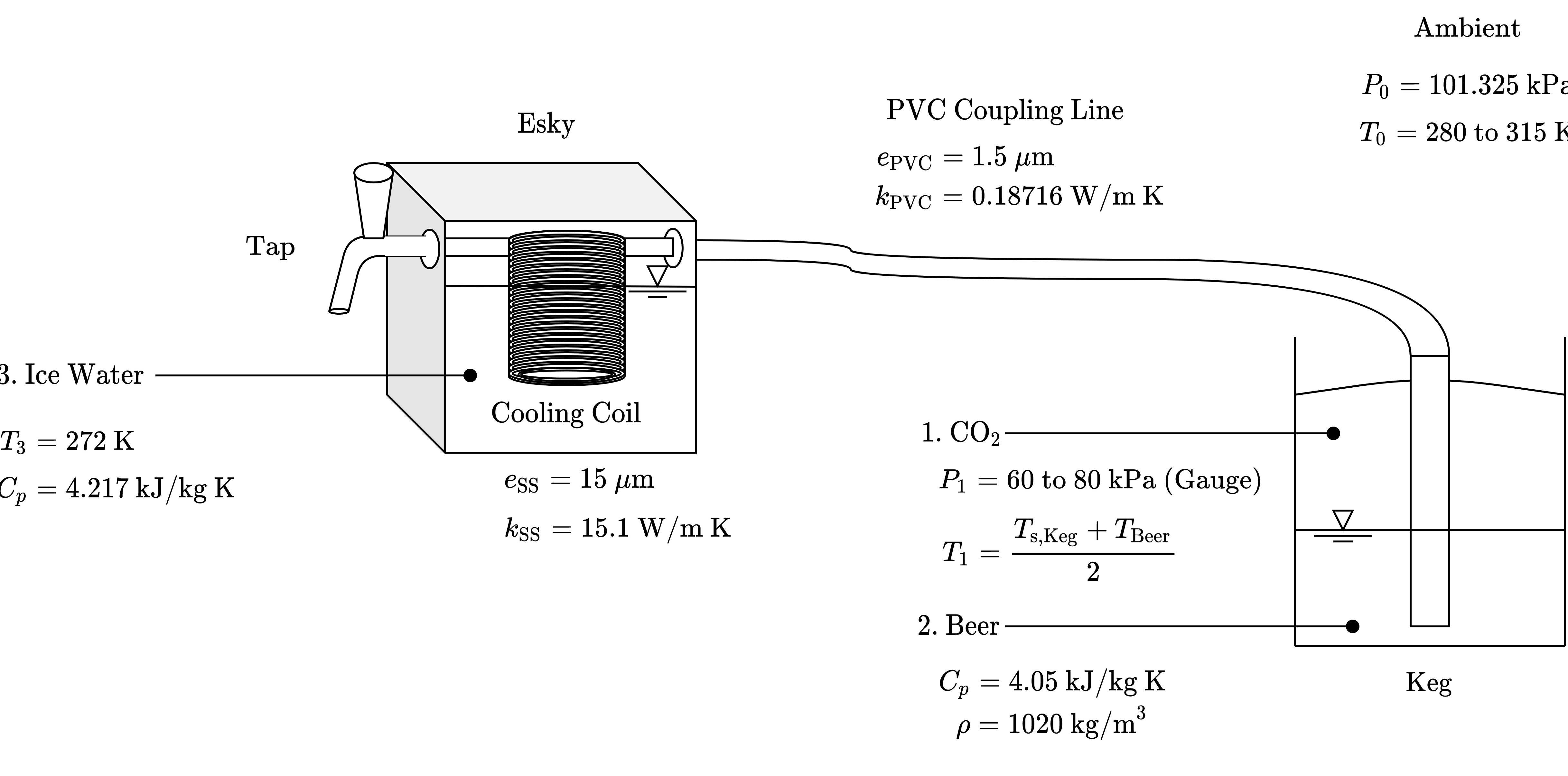
Fig. Schematic Diagram of Keg System

This is the general diagram locating key points of heat transfer in the system, ambient conditions and a setup for how the system operates from keg to tap. Analysing this shows the following regions will have heat transfer between the beer and other media:

CO₂ through the spear of the keg
Ambient air through the PVC coupling pipe
Ice water through the cooling coil in the esky

Given the system is relatively complex and the beer is carbonated, considering the flow characteristics of the system is also necessary to understand. The losses to the head of the system can be defined as follows:

Major frictional losses through the keg spear, PVC tubing and coil
Minor loss from re-entrant inlet on the keg spear and from angle valve on tap.
3 x minor losses from couplings through the system
20 x 2 (double layered) x 4 x 90° bends in coil

The major losses will need to be solved numerically from the Colebrook equation assuming turbulent flow, whilst the natural convection will be numerically solved for unknown surface temperatures.

Flow Characteristics

Given there a multiple diameters between the pipes in the system, the flow characteristics should be expressed in terms of the mass flow rate of the system, $\dot{m}$. This provides a solveable parameter which is common to each point in the system. It is necessary to produce an energy balance over the system, choosing a system boundary such that heat transfer does not form a part of the balance.

$$ \frac{V_2^2}{2}+\frac{P_1}{2}+gz_2 = \frac{V_\star^2}{2}+\frac{P_0}{2}+gz_\star + \sum h_f + \sum h_L $$

Eq. Fluid Flow Energy Balance

The star ($\star$) state indicates the exit from the tap. Rearranging this formulation allows for an expression in terms of the gauge pressure of the keg.

$$ \frac{P_{\text{gauge}}}{2} = g \Delta z + \frac{V_\star^2}{2}+gz_\star + \sum h_f + \sum h_L $$

Eq. Fluid Flow Energy Balance

The frictional losses, of the form $h_f = f \frac{L}{D} \frac{V^2}{2}$ can be expanded to be:

$$ \sum h_f = h_{f,\text{ PVC}} + h_{f,\text{ SS}} + h_{f,\text{ K}} $$

Eq. Major losses

where the friction factor $f$ of a pipe depends on the flow regime. Turbulent flows, depending on the roughness of the pipe can exhibit significantly higher or lower friction factors inhibiting their flow. To determine this, the Colebrook relation is used and determined based on the Reynold’s number in that pipe. If the flow is laminar, and below the critical Reynold’s number for internal flow (i.e $\text{Re} < 2300$) then a laminar approximation is to be used.

$$\frac{1}{\sqrt{f}}=-2\log{\left(\frac{e/D}{3.7}+\frac{2.51}{\text{Re}\sqrt{f}}\right)}$$

Eq. The Colebrook Equation

$$f = \frac{64}{\text{Re}}$$

Eq. Laminar Flow Approximation

Should the flow be laminar, a correction factor $\gamma$ is applied, where for laminar flows it is equal to 2, and for turbulent flows is approximately unity. This is applied to each $V^2$ term in the energy balance.

The minor losses are given to be:

$$ \sum h_L = h_{RE} + 3h_{C} + 160h_{90\text{°}} + h_V $$

Eq. Re-entrant, coupling, coil and valve minor losses

The re-entrant and coupling losses are both based off of a minor loss constant formulation of the form $h = K \frac{V^2}{2}$ whilst the 90° losses for the coil, and the valve are based on a characteristic length formulation $h = f_{\text{SS}} \frac{L_e}{D} \frac{V^2}{2}$.

Substituting all these values gives an equation in terms of the velocity at each point of interest in the fluid line. This is not solveable without a complementary equation reducing the unknowns. As mentioned previously, the mass flow rate must be a constant value given there is one inlet and one outlet to the system. Knowing the cross sectional areas at each analysis point in the system allows for the following substitution to be made:

$$ V = \frac{\dot{m}}{\rho_b A}$$

Eq. Velocity in terms of cross sectional area, density of beer and mass flow rate

Substituting this relation, gives the following equation to solve for the mass flow rate through the system.

$$ \dot{m} = \rho_b \frac{\sqrt{P_\text{gauge}+2g\Delta z}}{\sqrt{\frac{1}{A_\star^2}+\sum \frac{h_f}{A_i^2 V^2}+\sum \frac{h_L}{A_j^2 V^2}}}$$

Eq. Mass flow rate based on head of the system

The mass flow rate is related to the Reynolds number of the flow by the following relation. This allows for the mass flow rate to be iterated, converging on necessary friction factors, giving a converged mass flow rate for the system based on the pressure in the keg. This arrangement of the Reynolds number is given to be:

$$ \text{Re} = \frac{4\dot{m}}{\pi \mu_b D}$$

Eq. Reynolds number in terms of mass flow rate

Heat Transfer

This system is entirely dependent on external natural convection and internal forced convection in order to transfer heat from the fluid to the surroundings. The internal convection is related to the flow regime of the beer. In this case, if the flow is turbulent, the average Nusselt number is given to be:

$$ \bar{\text{Nu}}_D = 0.023 \text{Re}^{4/5} \text{Pr}_b^{0.3} $$

Eq. Nusselt number for internal turbulent flow

Otherwise, if the flow is laminar it can be assumed that the surface temperature of the tubes is constant (in thermal equilibrium) and the Nusselt number is hence constant ($\bar{\text{Nu}}_D=3.66$). The convection coefficient is hence derived by $\bar{h}=\frac{\bar{\text{Nu}}_D k_b}{L}$.

The external natural convection must be derived iteratively given an assumed surface temperature of the tubing at each stage. This assumed temperature is used to calculate an initial Raleigh number as per

$$ \text{Ra}_D = \frac{g \frac{1}{T_f}(T_s-T_\infty)D^3}{\nu \alpha} $$

Eq. Raleigh number

For the spear in the keg, the Nusselt number is calculated for the relating for a vertical cylinder

$$ \bar{\text{Nu}}_D = \left\{0.825+\frac{0.387\text{Ra}_D^{1/6}}{[1+(0.492/\text{Pr})^{9/16}]^{8/27}}\right\}^2 $$

Eq. Nusselt number for vertical tube

The PVC tubing and the coil are all assumed to be entirely horizontal in the reference frame. These Nusselt numbers are calculated slightly differently to the above:

$$ \bar{\text{Nu}}_D = \left\{0.6+\frac{0.387\text{Ra}_D^{1/6}}{[1+(0.559/\text{Pr})^{9/16}]^{8/27}}\right\}^2 $$

Eq. Nusselt number for horizontal tubing

The convection coefficient is calculated the same way as above. In this case, a value for the surface temperature of the tubing needs to be derived to iterated and improve the initial approximation. This is done by calculating the exit temperature of the fluid

$$ \frac{T_\infty - T_\text{ex}}{T_\infty - T_\text{in}} = \exp\left[\frac{-UA}{\dot{m}c_p}\right] $$

Eq. Equation to rearrange for exit temperature

This allows for the heat transfer to be calculated, using the total thermal resistance over the segment of flow $R_\text{tot}$

$$ \dot{q} = \frac{T_\text{in}-T_\text{ex}}{R_\text{tot}}$$

Eq. Heat flux

This then allows the average surface temperature to be derived noting the heat flux must still follow the thermal resistance formulation:

$$ T_s = T_\infty + \frac{\dot{q}}{\bar{h}A}$$

Eq. Surface temperature

Should this derived surface temperature be within a defined tolerance from the last value the system is assumed to be converged. The exit temperature at this position is used as the entrance temperature for the next segment of the system.

The exit temperature for the final segment corresponds to the serving temperature of the beer. The optimum temperature for a beer when served is anywhere between 6-9°C.

Code

You can find here a MATLAB implementation of the above with user defined inputs for the gauge pressure of the keg, temperature of the keg, air temperature and how full the keg is. Click here for a copy of the code.